How to convert expected goals into correct score probabilities with a Poisson model

Correct score betting rewards precise predictions but requires a statistical approach to avoid guessing. A simple and effective method is a Poisson-based model that converts each team’s scoring rate (or expected goals, xG) into probabilities for 0, 1, 2… goals. This part explains the core Poisson idea, how to estimate scoring rates, and practical adjustments for recent form, injuries and home advantage so bettors can produce usable score probabilities.

From expected goals to score probabilities: the Poisson basics

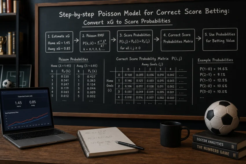
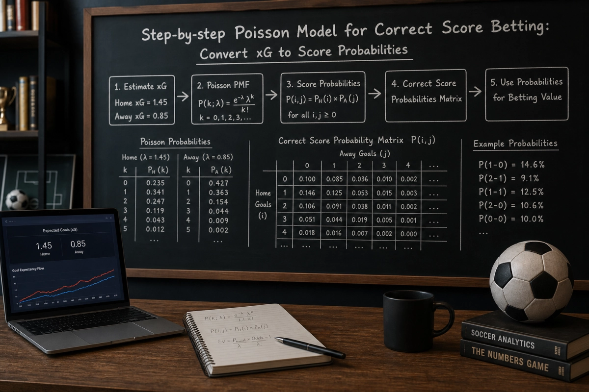
The Poisson distribution models the probability a team scores k goals given an average scoring rate λ (lambda). The formula is:

P(k goals) = e^−λ × λ^k / k!

To build a correct score matrix:

Choose λ_home and λ_away (expected goals for each team).
Compute P_home(k) and P_away(j) for k and j from 0 up to a reasonable cap (usually 4 or 5).
Assume independence and multiply: P(score k–j) = P_home(k) × P_away(j).

Example (conceptual): if λ_home = 1.5 and λ_away = 0.9, the model gives probabilities for 0–0, 1–0, 0–1, 2–1 etc. Summing relevant cells also yields probabilities for markets like match result, over/under goals and both teams to score.

Why cap goals and how to handle tails

Practical models compute probabilities for 0–4 or 0–5 goals and treat any higher score as “5+” or distribute the small tail probability proportionally. This keeps computation simple while capturing the meaningful mass of the distribution.

Adjusting scoring rates: form, injuries and home advantage

Raw historical averages or xG numbers are a start, but bettors should adjust λ for current context:

Recent form: Weight recent matches more heavily (for example, using an exponential decay) because teams change over time.
Injuries and suspensions: Reduce or increase λ depending on the absence/presence of key attackers or defenders. If a leading scorer is out, reduce the team’s attacking λ; if a key keeper is missing, increase opponent λ.
Home advantage: Apply a multiplicative factor to the home team’s λ (commonly between 1.05–1.20 depending on league and sample data) and the inverse to the away team if data supports it.
Tactical matchup and motivation: Consider styles (counter-attacking vs possession), fixture congestion, and competition stakes—these are qualitative but can justify small λ adjustments.

Always document adjustments and avoid overfitting: make small, consistent tweaks rather than large one-off changes based on speculation.

Limitations to bear in mind

The Poisson model assumes independence of team goal events and constant rate during the match—both simplifications that can fail for some fixtures.
Low-probability, high-goal games are poorly modelled unless you expand the goal cap or use alternative distributions (negative binomial, bivariate Poisson) later.
Adjustments rely on judgement; inconsistent or extreme changes introduce bias.

Quick guide to related betting markets and how probabilities map to odds

From the correct score matrix you can derive probabilities for match result (1X2), both teams to score (BTTS), over/under goals, Asian handicap and more. To compare with bookmakers:

Convert bookmaker odds to implied probabilities (1 / decimal odds) and adjust for the book’s margin.
Look for value where model probability > market implied probability.

In the next section the article will show a worked example—calculating λ from data, producing a full correct score table, comparing model probabilities with market odds and outlining staking considerations for correct score betting.

Worked example: calculate λ, build the correct‑score table and read key cells

Start with estimated expected goals (λ) for the match—after applying your adjustments for form, injuries and home advantage. Using the earlier example: λ_home = 1.5 and λ_away = 0.9. Compute Poisson probabilities for k = 0…4 (you can cap at 4 and treat the tail as 5+).

Home (λ = 1.5)
– P(0) = e−1.5 = 0.22313
– P(1) = 1.5 × e−1.5 = 0.33470
– P(2) = 1.5^2/2 × e−1.5 = 0.25102
– P(3) = 0.12551
– P(4) = 0.04707

Away (λ = 0.9)
– P(0) = e−0.9 = 0.40657
– P(1) = 0.36591
– P(2) = 0.16466
– P(3) = 0.04940
– P(4) = 0.01111

Assuming independence, multiply the corresponding probabilities to populate the correct‑score matrix. A few example cells:
– P(1–0) = P_home(1) × P_away(0) = 0.33470 × 0.40657 ≈ 0.1361 (13.61%)
– P(1–1) = 0.33470 × 0.36591 ≈ 0.1224 (12.24%)
– P(2–0) = 0.25102 × 0.40657 ≈ 0.1020 (10.20%)
– P(0–0) = 0.22313 × 0.40657 ≈ 0.0907 (9.07%)
– P(2–1) = 0.25102 × 0.36591 ≈ 0.0918 (9.18%)

From the full matrix you can (a) identify the most likely exact scores, (b) sum cells for markets like 1X2 or BTTS, and (c) calculate the cumulative probability for “5+” by summing your treated tail cell(s).

Document the λ values and the adjustments you made so you can backtest or iterate later.

Compare model probabilities with market odds and staking guidance

Convert bookmaker decimal odds to implied probabilities (implied = 1 / decimal odds). Because books include a margin, you should normalize the set of implied probabilities across the correct‑score market (divide each implied probability by the sum of all implied probabilities) to get a margin‑adjusted market probability for each exact score.

Example check for a single cell: if the book offers 7.5 for 1–0, implied = 1 / 7.5 = 13.33%. Your model gives 13.61% for 1–0, so raw model > raw market (a small edge). After removing overround the relative edge will change slightly, but the sign and magnitude give you a quick sense of potential value.

Staking: correct score wins are high‑variance, so apply conservative staking. Use fractional Kelly rather than full Kelly. Kelly fraction for a single bet:
– f* = (b × p − (1 − p)) / b, where b = decimal odds − 1 and p = your model probability.

Using the 1–0 example (p = 0.1361, book decimal = 7.5 → b = 6.5):
– f* ≈ (6.5×0.1361 − 0.8639) / 6.5 ≈ 0.0032 → ~0.32% of bankroll (full Kelly).
A practical choice is 1/4 Kelly (≈0.08% here) or a small flat stake (e.g., 0.25% of bankroll) to reduce volatility and model risk.

Other staking rules
– Cap single bets (e.g., max 1%–2% of bankroll) to avoid blowups.
– Avoid betting many correlated correct‑score markets on the same slate.
– Track results and adjust your model: small persistent discrepancies may indicate a systematic bias.

Finally, be realistic about expected edges: correct‑score inefficiencies exist but are typically small and require volume, disciplined staking, and accounting for limits, commissions and bookmaker behavior. Part 3 will cover detailed backtesting, model calibration and practical shortcuts to scale this approach.

Putting the model into practice

Use the Poisson approach as a disciplined workflow rather than a promise of guaranteed profit: document your assumptions, log every adjustment, and treat each bet as a test of the model. Small, repeatable steps and careful record‑keeping are what turn a statistical edge into long‑term results.

Quick pre‑bet checklist

Record the λ values and the reason for each adjustment (form, injuries, home factor).
Normalize bookmaker implied probabilities across the correct‑score market to remove overround.
Compare model probability to market probability and calculate stake using a conservative Kelly fraction or a capped flat stake.
Limit exposure per bet (commonly ≤1% of bankroll) and avoid multiple correlated bets on the same fixture.
Log stake, odds, model probability and result for ongoing calibration and performance tracking.

Caveats and responsible practice

Expect high variance: even edges can look poor over short samples. Patience and volume matter.
Bookmakers act on profitable patterns—liquidity limits and account restrictions are real constraints.
Model assumptions (independence, constant rate) are simplifications—monitor where they fail and consider more advanced models if necessary.
Avoid overfitting: keep adjustments transparent and test them out‑of‑sample before increasing stakes.
Practice sound bankroll management and never bet money you cannot afford to lose.

Keep refining the model, be honest about its limits, and let disciplined process and data — not emotion — guide your betting decisions.